monticello // Shutterstock

10 Google Sheets hacks that will make your job easier

Google’s free-to-use software is ubiquitous in today’s corporate world, whether you’re employed at a large or small firm. So why aren’t you a pro at it yet?

In 2020, Google shared that its suite of productivity tools, including Gmail, Google Docs, and Google Sheets—Microsoft’s Excel software competitor—had surpassed 2 billion monthly users. Like everything else in Google’s software suite, Google Sheets syncs automatically with multiple users so you and others can collaborate seamlessly. It is perhaps the most accessible and powerful piece of software available today for workers wanting to wrap their hands around large sets of data.

Whether for work or simply for budgeting in your personal life, developing a stronger grasp of the shortcuts available in Google Sheets is an easy way to save time better spent on something besides hunching over a keyboard.

ClickUp scoured the most-followed social media influencers sharing spreadsheet tips and tricks, including CheatSheets and Your Excel Dictionary, to compile this list of ten Google Sheets hacks you should be putting in rotation.

Start by bookmarking this artificial-intelligence-enabled tool called Excel Formulator, which lets users dictate what they want a Google Sheets function to do and spits out the function—and keep reading for more helpful tips.

ClickUp

Quick-and-dirty charts

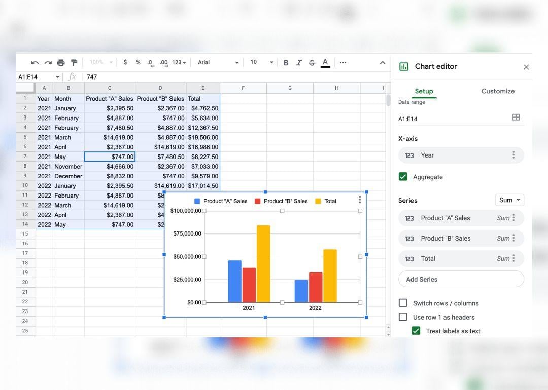
Heading into a meeting and need to grab a quick trend line so you know what you’re talking about? In Excel, you would use Alt + F1, or Option + F1 on a Mac, after selecting a data table to generate a quick chart of the data you have selected. In Google Sheets, you’ll need to use your mouse not just to select your table but also to select “Chart” from the “Insert” drop-down menu.

ClickUp

Add everything up in a second

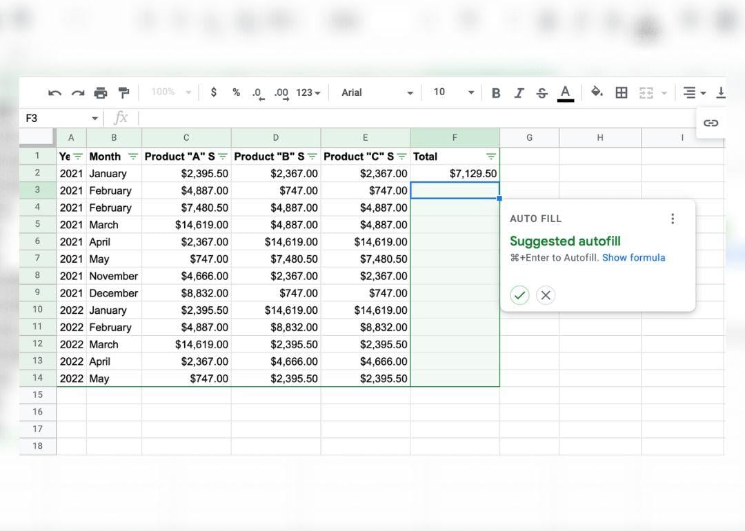
In Excel, selecting your data with Ctrl + A and then using Alt + = will run the Sum function for an entire data table if the table is formatted in a standard way. Google’s spreadsheet processing software attempts to make this easier by sensing when to automatically fill in a function.

You should only need to enter a function once before getting the autofill prompt. This is helpful for the commonly used =SUM function, which will add up all of the values in the preceding rows for you.

Google Sheets functions a little differently, and you may have an easier time prompting it to autofill functions after you create a filter view. Simply click the filter button on the far right of your toolbar and select “Create new filter view” to enable this.

ClickUp

Split up messy data or lists into nice columns

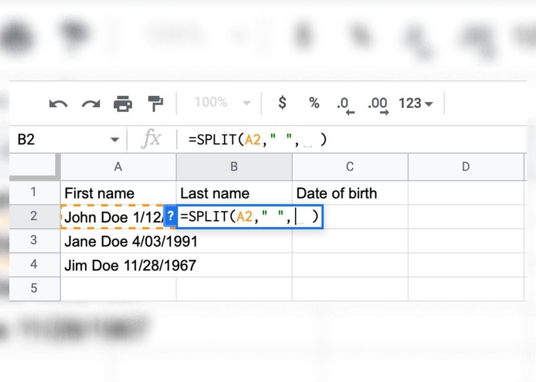
The =SPLIT function lets you split up a cell’s data on the character you put within the quotation marks.

ClickUp

Hide those ugly errors

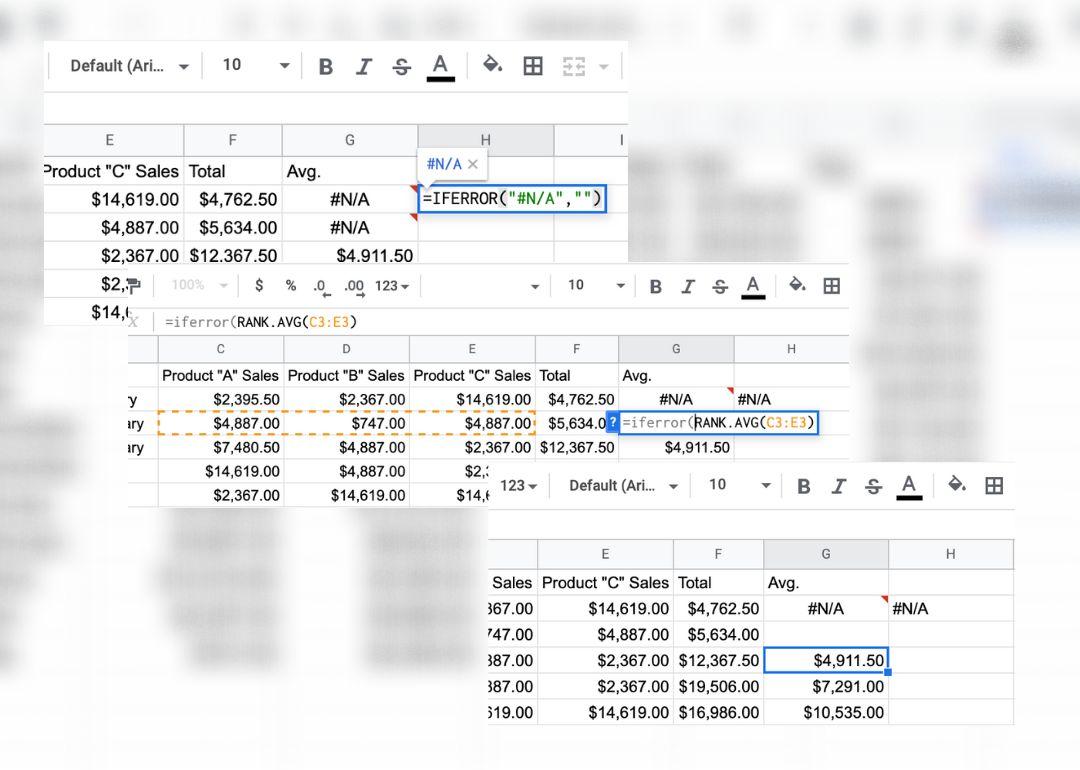
The =IFERROR function allows you to tell the spreadsheets to recognize any errors and display whatever values you place between the quotation marks—including blank space if you prefer. This requires that you write all of your formulas nested within the =IFERROR( expression’s parentheses.

ClickUp

Auto-size your data

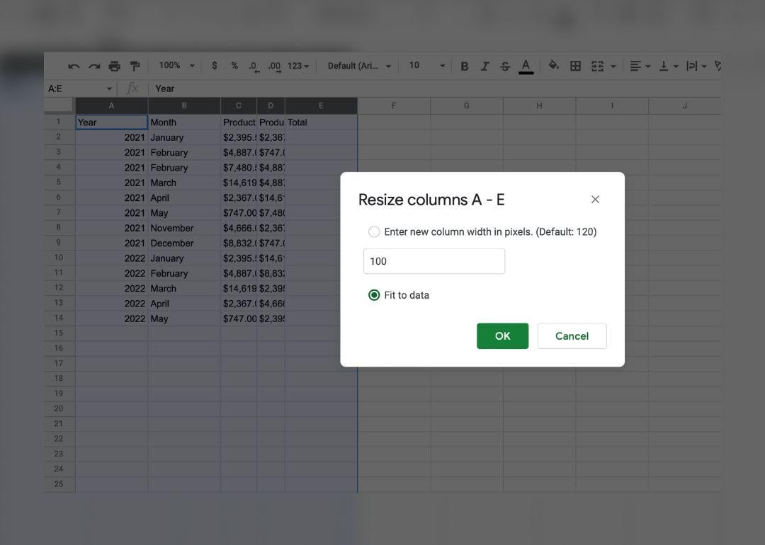
Are your columns and rows making it hard to see the full value in each cell? There are two ways Google Sheets gives us to fix this. First, you can right-click a column or row and select “Resize column” or “Resize row,” then choose “Fit to data” and click “OK.”

A quicker shortcut is to double-click the line separating the row or column, and it will snap into the perfect size for the values it contains.

ClickUp

Fill your columns automatically

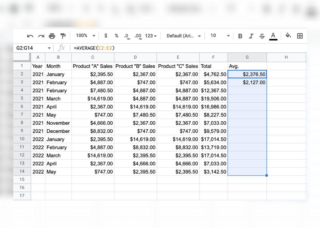
The next time you need to enter a series of dates or copy a formula, enter the first two, then stop. Use the Ctrl + D key combination, or Command + D if you’re using a Mac, to fill a column down. Google Sheets will guess and fill in the rest of the dates or other figures based on the patterns it recognizes in your row or column. You can also use Ctrl + R or Command + R to fill a column to the right. This is also called “flash fill.”

ClickUp

Import data straight from webpages

Quit copying and pasting poorly-formatted tables from webpages.

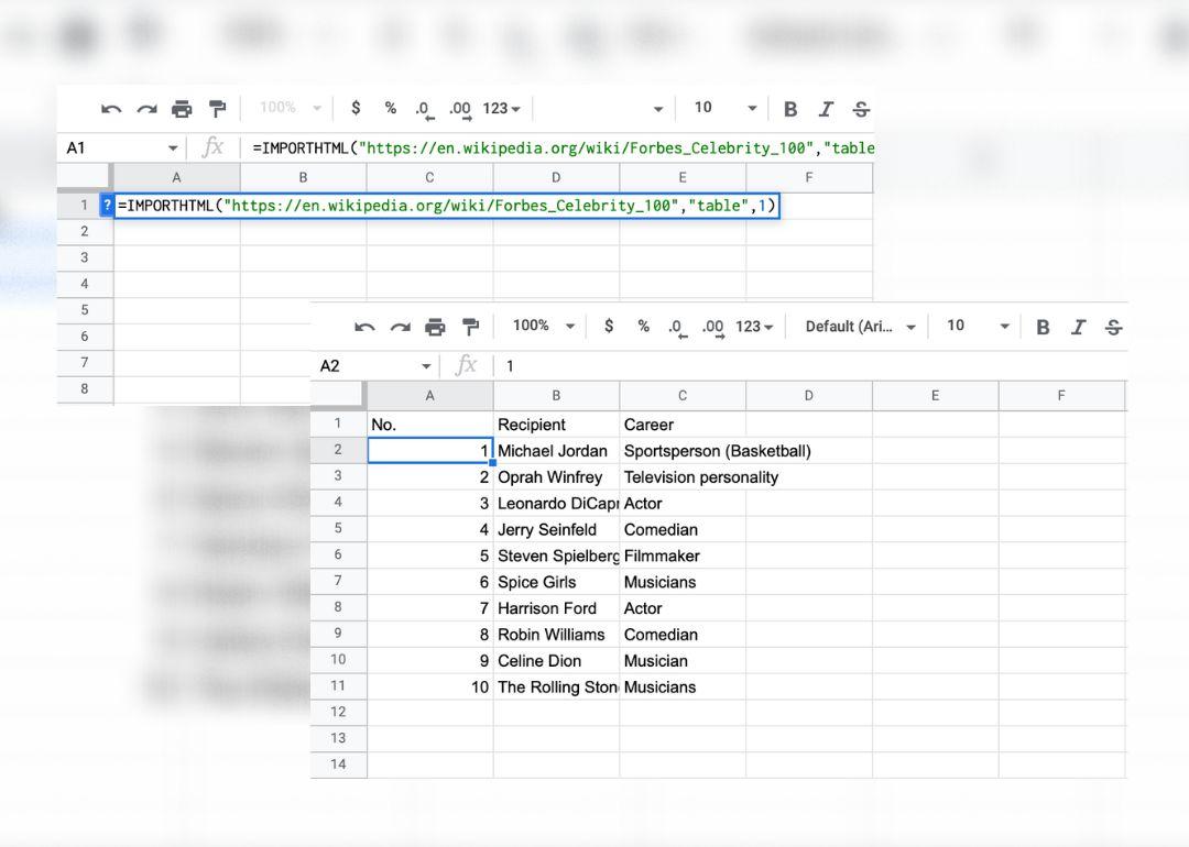
You can enter the =IMPORTHTML function in Google Sheets to import a table or list from a webpage you’ve copied the URL from. Include “table/list”, “1” in the function to grab the first table. It’s important to note that not every data source will import nicely. If your import doesn’t work the first time, make sure there are quotation marks around each component, including the URL.

ClickUp

Create buttons to hide and reveal certain things

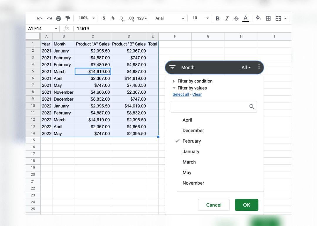
You can utilize the Slicer function to look at “slices” of your data set. Highlight the data and choose “Add a slicer” from the “Data” drop-down menu. From there, you can choose which identifiers you want to show through when you turn the slicer on and off with a click.

ClickUp

Clean up capitalization and spacing

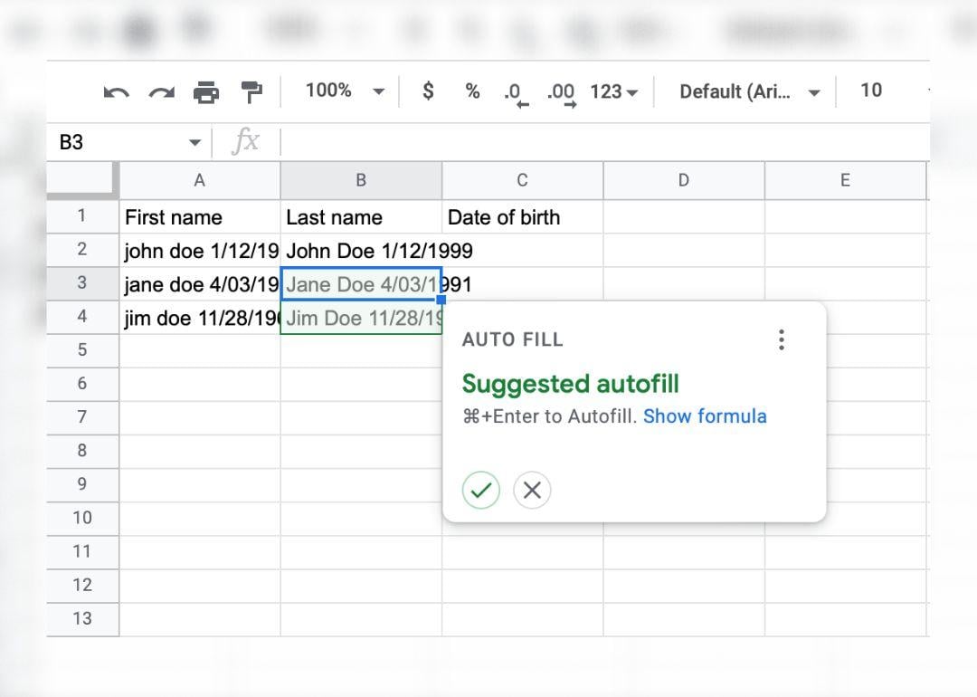
Try using =PROPER(insert cell containing values here) to capitalize poorly formatted text in a flash. You can also nest the trim function in here as =TRIM(PROPER(insert cell containing values here) to remove pesky unwanted spaces.

ClickUp

Automatically change a cell’s color based on the value

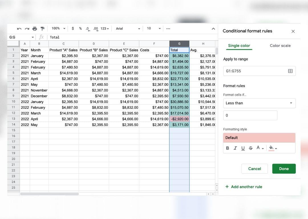
Use conditional formatting to create rules for a column or row of data. You can have cells in that range turn colors based on a word, character, or positive or negative value. One of the most obvious applications for this includes coding cells to turn green or red for positive and negative change across data sets.

This story originally appeared on ClickUp and was produced and
distributed in partnership with Stacker Studio.